Diffusion Policy: 将扩散模型加噪-去噪的看家本领用于生成机器人动作啦！

开场白

之前写 diffusion model 的吹水文，都是聚焦在 CV 领域，这次来玩点新东西——Robotics，毕竟 CW 不要无聊的风格嘛~ 本文的主角是：Diffusion Policy: Visuomotor Policy Learning via Action Diffusion(https://arxiv.org/abs/2303.04137)，虽然如今算是老家伙了，但在当时貌似也是流量小明星一枚。

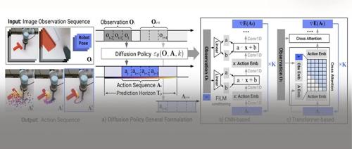
何谓 Diffusion Policy？用作者的话说就是：a new way of generating robot behavior by representing a robot’s visuomotor policy as a conditional denoising diffusion process.

嗯，相信各位玩家们都已经知道这是怎么玩的了。就是把扩散模型拿到机器人领域玩，在图像生成里是对图像加噪来建模图像分布，搬到这里来就是对动作加噪来建模动作分布(简直写轮眼了~)。

话说人家扩散模型本来是搞视觉生成的，随着现在的打工人越来越卷，它也是被迫打了好几份工，什么文本生成、语音生成、蛋白质生成以及本文这里的机器人动作生成，哪哪都有它。可能怪就怪在它的玩法过于简(无)单(脑)直接吧——想要生成什么目标就对它加高斯噪声，然后去学习预测噪声就完事儿~

虽然好久不见，不过 CW 依旧会秉持一贯不无聊的风格——先吹吹水，动动嘴；再进行代码实现，动动手。

话不多说，下面正式进入正文~！

Keywords: Imitation learning, visuomotor policy, manipulation, diffusion model

任务特性

机器人决策(预测动作)任务有着其独特性质和要求，这些方面使得大家在炼丹时会面临一些挑战，于是需要仔细考虑不少因素并进行相应的设计，下面就列举一些这项任务所拥有的“特点”：

“多模态”

多模态分布意味着在相同的观测情况下，可能存在多种合理的动作选择。这种多模态性增加了模型学习的复杂性，因为它需要考虑到多种可能的输出，而不是单一的确定值。

序列相关性

序列相关性是指机器人的动作之间存在依赖关系。机器人前一个动作的执行结果会影响到下一个动作的选择。模型需要捕捉这种序列相关性，才能生成连贯、有效的动作序列。

高精度

在诸如手术机器人、精密装配机器人等应用场景中，微小的动作偏差都可能导致严重的后果。这就要求模型在学习观测 – 动作映射时，必须达到极高的准确性，这对模型的学习能力和泛化能力提出了很高的要求。

背景与动机

要让机器人学会根据当前观测状态做出合理的决策，最简单直接的做法就是根据演示(demonstration)来学习策略(policy)，这属于监督学习的方式，它期望在观测状态(observations)和动作(actions)之间建立有效映射，其核心思想是让模型通过观察人类或其他智能体的演示行为，学习如何在不同的观测情况下做出合适的动作(嗯，照葫芦画瓢~)。但由于机器人的动作预测具有以上特点，因此使得这项任务与其他监督任务相比更具有挑战性。

以往的做法

为了应对这些挑战，业界不乏各种卷王提出了各种方法，以往的这些方法大致分为两类：

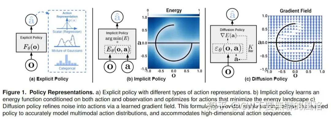
• 显式策略

如上图(a)所示，直接将动作表示(action representations)建模为某种特定的分布，比如：将连续的动作空间划分成多个离散的类别，从而建模为分类分布(categorical distribution)；或者建模为混合高斯分布，通过调整其中个各高斯分布的比重，便可以灵活地改变动作选择的多样性，从而应对以上提到的动作分布的多模态特性；还有的就是简单粗暴地直接对目标动作进行回归(regression)。

• 隐式策略

前面提到的显式策略简单直接——直接将观测状态映射到动作，但在应对多模态动作分布时容易凸显出局限性(很难覆盖到所有合理的目标动作)。于是，就有了如上图(b)所示的隐式策略——通过学习一个能量函数，以观测状态和动作为输入，输出对应的能量值，越优的动作对应的能量值越小。这种策略将动作预测转化为寻找使能量值最小的动作，它不直接输出动作，而是基于输出的能量值来对动作进行选择，因此称其为“隐式”策略。由于同样的低能量状态可能存在多个对应的动作，因此可以有效捕捉动作表示的多模态特性。

存在的问题

以上策略都具有一些毛病：

在显式策略中，基于回归的方式直接将观测状态映射到动作，缺乏校正的余地和灵活性，难以应对高精度任务，且通常只能捕捉到单一的动作，从而忽略其它合理动作。

而将回归任务转换为分类任务，通过离散化动作空间来处理多模态分布，又会使逼近连续动作空间所需的类别数量随维度增加呈指数增长，导致计算复杂度大幅提高。

对于混合高斯策略，它会随着动作空间维度的增加和多模态分布复杂性的提高，而需要更多的高斯分量来准确表示分布，这会使模型参数数量大幅增加，导致模型复杂度呈指数级上升，推理过程时计算量也会显著增大，可能使实时性难以满足要求。

至于隐式策略嘛.. 炼丹师们都懂——它不好训呀！计算 Info-NCE 损失(需要估计归一化常数)需要抽取负样本，而这种做法会使得估算的归一化常数不准且可能变动极大，从而导致训练很不稳定。

Anyway, 以上这些家伙都无法很好地应对上一节提到的序列相关的特性。

正片开始

这又不行，那又不行的，只能自己整活咯~

下面就正式将聚光灯洒在本文主角——diffusion policy 身上！

建模方式

鉴于之前的那些家伙都不太行，作者决定“自力更生”，推出了一种新的建模方式：

generates behavior via a “conditional denoising diffusion process on robot action space”

与显式策略不同，这种方法不是直接输出动作，而是输出动作分布的条件得分函数(score function)，以视觉观测(visual observations，通常是表示当下情况的图像)为条件，然后像去噪扩散模型一样，在经历迭代去噪过程后最终才输出目标动作。

讲人话就是，仿照扩散模型学习图像生成的套路——训练时对目标动作加噪，然后模型预测所加的噪声，最终学会建模动作空间分布。虽然论文一直说模型学习/预测的是 score function，但实际上作者采取的是 DDPM 那种预测噪声的做法。不过没毛病，随着炼丹界大一统进程的发展，大家都清楚本质上扩散模型、分数模型 以及 flow-based 这些家伙们其实都是一家人。

继承

自然地，这种玩法继承了扩散模型的一些优点：

• 能够建模多峰分布

在提出分数模型(Score Network)(https://arxiv.org/abs/1907.05600) 的 paper 中已经论述过，通过让模型学习得分函数，并根据朗之万动力学(Langevin Dynamics)(https://friedmanroy.github.io/blog/2022/Langevin/)进行采样，结果能够覆盖到多峰分布(对应 diffusion policy 论文中所谓的 “multimodal”)，从而能够捕捉到多种合理动作。

• 轻松处理高维输出空间

扩散模型能够在视觉生成领域大放异彩，那么它理所应当是能够轻松 handle 高维空间数据的。利用这种特性，diffusion policy 就能够在一次预测中输出一个动作序列，而非单步动作，这对于维持前后动作的一致性(temporal action consistency) 相当重要，并且能够避免“目光短浅”的预测行为——也就是能够考虑到多个时间步而实施长期规划。

• 训练稳定

由于模型学习的是得分函数，规避了学习能量函数所须估算归一化常数(which is intractable)的麻烦(会导致训练不稳定)，因此 diffusion policy 的训练稳定性会相对友好些~

发扬

以上方面都是继承自扩散模型，而作为“后生仔”总得自己搞一些事情。于是，为了将扩散模型有效应用到机器人的视觉策略学习(visuomotor policy learning)中，作者还应用了以下几项关键技术：

• receding-horizon control

这种叫 “Receding-Horizon Control(RHC)”的玩法源于控制系统，也就是做决策前需要考虑到未来的不确定性和变化，以便在每个时间步上重新调整策略。

得益于扩散模型在高维空间上的表现，diffusion policy 可以一次性预测一个序列的动作，作者将这个特性与 RHC 相结合，使得动作执行更加鲁棒(robust)，这种设计使策略能够以闭环的方式持续地重新规划其动作，论文中称之为 “closed-loop action sequences”.

概括来说，就是根据当前(及过去)的系统状态，一次性预测 T_p 步的动作，但仅执行其中的 T_a (T_a < T_p) 步。剩余未执行的部分就“留有了重新规划的余地”，接下来智能体就可以基于新的系统状态重新进行规划和预测。不断持续这样做，从而形成一个闭环优化和调整的过程(具体细节看后文代码实现部分会有更清晰的认知)。

照这么玩，diffusion policy 就既能够进行长期的动作规划，又能在遇到突发状况时进行策略调整，兼顾了长期规划和实时响应能力，从而保证了系统运行的稳定性和可靠性。

• visual conditioning

将体现当前观测状态的图像作为条件输入到扩散模型去辅助做决策(如文生图的玩法一般)，输入前会先将图像喂给图像编码器(比如 ResNet 之类的)编码为特征。

• Time-series diffusion transformer

引入了一种 Transformer 结构的扩散模型(不是 DiT, 那时候 DiT 还没有出生呢~)，这是因为作者发现，CNN-based 的扩散模型(如典型的 U-Net 架构)有过度平滑(over-smoothing)的效应，在应对一些需要突然大幅改变动作(high-frequency action changes)的任务时不太给力。这也容易理解，毕竟卷积本身就是一种平滑滤波。

关键设计

为了让 diffusion policy 在舞台上大放光彩，作者煞费心思地在模型和算法方面做了一些关键设计，下面就一起来看看叭~

网络架构

• CNN-based

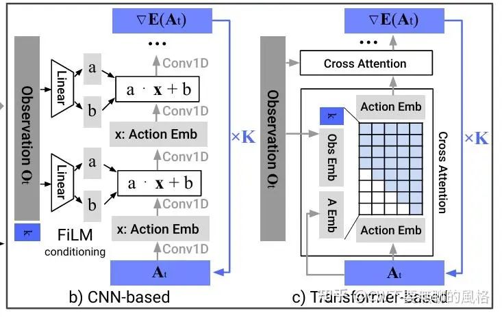
作者参考了 Planning with Diffusion for Flexible Behavior Synthesis(https://arxiv.org/abs/2205.09991) 这篇 paper，采用 1D 时序 CNN 去建模条件分布 分别代表观测状态和动作。与此同时，作者还将加／去噪迭代轮数  与观测状态  相结合作为条件，并利用 FiLM(https://arxiv.org/abs/1709.07871) 技术注入到扩散模型中。具体做法如上图 b）所示，实质就是将条件向量输入到 Linear 层生成 scale \＆shift 参数  ，然后对主特征  进行调制： .

在实践中，这种架构不需要太费劲去调参就能够胜任许多任务。不过，如前文提到的那样，当面临那些目标动作序列是高频变化或者大幅改变的情况时就 GG 了，作者觉得这可能是时序卷积拥有偏好低频信号的归纳偏置(https://arxiv.org/abs/2006.10739)所致。

• Time-series diffusion transformer

为了克服以上架构的不足，作者参考 Behavior Transformers: Cloning k modes with one stone(https://arxiv.org/abs/2206.11251) 这篇 paper 采取了 Transformer 架构 (decoder-only) 。在这种架构下，带噪声的动作序列  作为 input tokens，加／去噪迭代轮数  通过正弦编码为 embedding 向量，观测状态  则通过 MLP 转换成 embedding 序列。随后  与  通过 cross attention 进行交互，其中使用 causal mask 使得每个动作只能看到自身及之前的位置，如上图 c）所示。

相比于 CNN-based，这种架构的上限虽然更高，但却对超参更加敏感。不过，作者看到 Understanding the Difficulty of Training Transformers(https://arxiv.org/abs/2004.08249) 这篇 paper 后，也就安了，原来不是我一个人的问题(偷笑~)。

此外，作者还给出了温馨建议：当你首次尝试一个新任务时，建议使用 CNN-based 架构，若搞不定，并且发现这是因为任务过于复杂或者是其中需要高频快速地改变动作，那么你就可以转用 Transformer 架构，然后玩命炼丹即是(因为可能要很努力地去调整超参)。

CW 灵魂拷问：若 CNN-based 架构搞不定，但任务本身简单，并且不要求高频改变动作，那..？

视觉编码器

视觉编码器用于将观测图像编码为 latent embedding O_t ，默认选用 ResNet-18，但需要重新训练或者以小的学习率(通常比扩散模小10x)进一步微调，而不是直接使用预训练权重并固定住，因为作者发现那样效果会不好，说明机器人动作预测任务所需的视觉特征与在 ImageNet 这种图像识别任务上学到的特征存在一定的 gap。另外还需要注意的是，作者使用的并非原版 ResNet-18，而是 DIY 了一下：

(i). 将全局平均池化(global average pooling) 改为 spatial softmax pooling(https://arxiv.org/abs/2108.03298) 以保持图像空间信息；

(ii). 将 BatchNorm 改为 GroupNorm 以便让训练更稳定。作者说，当在训练期间使用 EMA(Exponential Moving Average) 时，这么做特别重要。

另外，当存在多个摄像头去捕捉观测图像时，不同的摄像头会使用独立的视觉编码器，最后再将它们各自的编码结果 concat 在一起作为 .

噪声调度方案

扩散模型的玩家们都知道这是啥东东，这里就不再多说什么了。作者使用的是在 iDDPM(https://arxiv.org/abs/2102.09672) 那篇 paper 中提出的 Square Cosine Schedule ，因为经过实验检验，这种方案效果最好。

加速采样

为了满足实时性需求，采用 DDIM(https://arxiv.org/abs/2010.02502) 进行采样，以减少原来 DDPM 的采样步数。经过真实场景下测试，在单张 3080 上达到 0.1 秒的推理延迟。

特性和优势

这一章来盘点一些 diffusion policy 这个方法所拥有的一些特性和优势。优不优 CW 不敢确定，反正从作者在论文中的表述来看，至少评个三好学生是没问题的~

多模态的动作分布

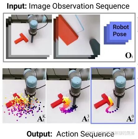
如上图所示，diffusion policy 能够表现出多模态的动作分布，这归因于其采样过程的随机性以及随机的采样起点。采样起点  是随机的高斯噪声，这导致最终可能会走向不同的目标动作  ．并且，朗之万动力采样会在每步迭代中添加高斯噪声扰动，这使得各个动作能够在不同的模态域之间移动并收敛。

基于位置控制的动作空间

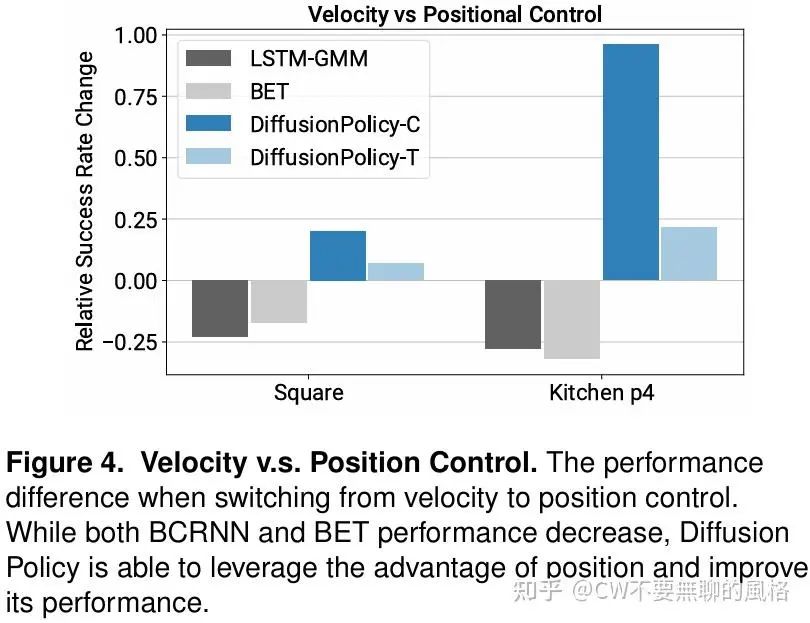
作者通过实验发现，使用位置控制(position-control)的动作空间比速度控制(velocity control)来得更优，这与之前的一些 paper 的结论相矛盾，作者认为这可能有以下原因：

1. 使用位置控制能够更好地表现动作的多模态特性，因为这种方式只关注目标位置，而对于中间过程没有太多约束，所以为“通过多种路径抵达终点”带来了可能性。相反，速度控制的方式则相当于在路径上实施了较为严格的约束。

2. 使用速度控制的方式会有累积误差效应，因为位置是路径速度的积分，所以其中每一步的误差会被累积，后续时刻的位置会继承先前的并不断叠加。这种方式更加注重局部状态的反馈(当前每步实际与目标速度的差异)，而使用位置控制的方式相当于使用全局状态(最终位置)作为反馈目标，更易对误差进行修正。

预测动作序列

有了扩散模型的加持，diffusion policy 能够轻松 handle 高维空间的输出，于是作者就进一步利用这个优势去预测动作序列 (即多步而非单步动作) 。然而这种预测序列的玩法是以往很多方法所忌讳的，因为它们难以高效地从在高维的动作空间中进行采样(说的就是你们：IBC, BC-RNN, BET)。

此外，这种玩法还享有以下好处：

• temporal action consistency

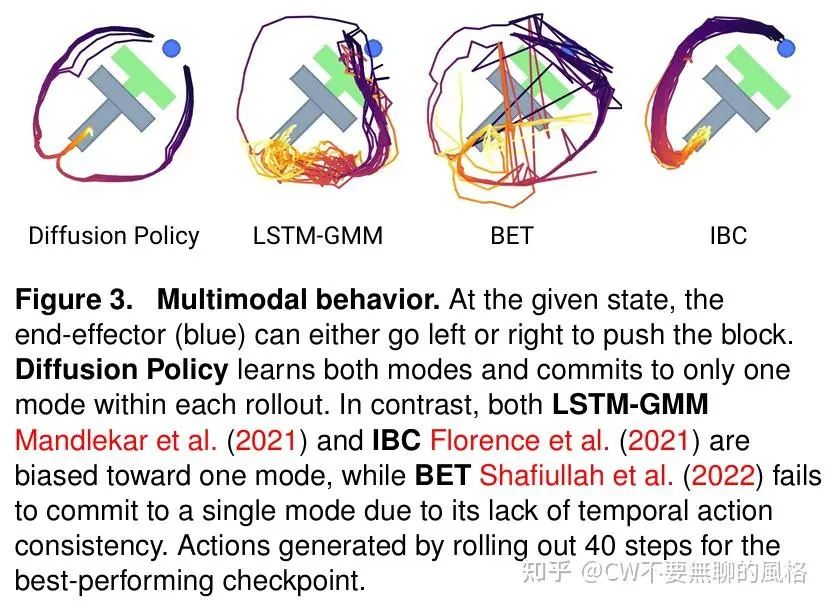
也就是前后动作拥有一致性，不会前后矛盾。如前面图3所示，虽然 diffusion policy 能够表现出多模态的路径选择，但一旦选择了一条路径后就会“一致地走下去”直至完成目标，不会像 BEC 那般“反复横跳”，一下走这条路另一下又切换到另一边去了，这是因为它相当于将每步的动作都视作独立的，没有考虑到彼此。而 diffusion policy 每次预测的都是一整个动作序列，每个动作之间会相互“兼顾”。

• robustness to idle actions

有些任务比如倒液体这种，在某段时间内要求位置不变/速度接近于0，但机器人有时候就会“短路”地以为要一直这样不动，永生永世.. 当训练数据中包含像这样的 “idle actions” 时，像 BC-RNN 和 IBC 之流在实际场景中就容易一直尬住(是的，又点名批评啦！)，因为它们只考虑了单步动作，没有看到全局，而 diffusion policy 每次都看一整个序列，容易识破这种 idle 状态只是一个过渡的过程，并非“最终归属”。

训练稳定

给张图你们自行感受下：

IBC 这抖成 dog 的 loss 比我邻居姥爷的腿还抖，再看看本文主角——diffusion policy 的，犹如一道亮丽的风景线划过，搞得 CW 都不由地还唱出了陈奕迅歌词里的那句：天空闪过灿烂花火(猜歌名，有奖hhh)~

IBC 的 loss 之所以如此＂飘忽不定＂，是因为 EBM（Energy－Based Model）这类模型的建模方式是： ，其中  是 intractable 的归一化常数。由于这个常数实际不可求，因此在实际训练时会使用  对其进行估计，这就需要通过采样一堆负样本  来完成，然后再结合 InfoNCE－style 的损失函数：

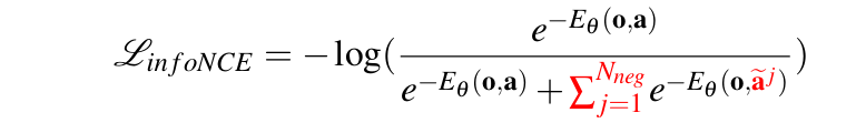
由于不可能穷尽所有可能的负样本，因此每次采样的方差可能很大，估计的偏差也可能大，最终就导致 EBM 的训练不稳定。

然而，扩散模型学习的是 score function：

它是目标动作的导数，由于与归一化常数无关，因此相关的导数项为0，这就幸运地与那个难搞的归一化常数撇清关系啦(^_^)~！可以看到，diffusion policy 无论是训练 loss 还是推理时的成功率，画出的曲线都像是亮丽的风景线，看起来十分舒服~

神马！？不了解 score function？那请速度来了解下 CW 的考古吹水文：

https://zhuanlan.zhihu.com/p/597490389

局限

没有盲目自信，作者在论文中点出了 diffusion policy 的一些不足与局限。

首先是继承了行为克隆(behavior cloning)这类方法本身所拥有的局限性，毕竟本质上 diffusion policy 也是“照着课本念书”——根据演示数据进行监督学习。当演示数据量不够充分时，训练得到的性能就不太能打，泛化性也不够强。于是大家自然容易联想到——若引入隔壁班的强化学习的话，应该会有所改善。

其次就是由于扩散模型是迭代去噪的采样过程，因此与 LSTM-GMM 这类朋友相比，就带来了更高的计算消耗和推理延迟。咦，diffusion policy 这不又是继承了别人(i.e. 扩散模型)的糟粕..？对此，作者在论文中提到，可以采用更先进的采样算法来减少采样步数，比如宋飏大佬提出的 一致性模型(Consistency Model)(https://arxiv.org/abs/2303.01469)。哦，原来 Ilya也是作者之一，WOW~ 豪华阵容！

Workflow

前面讲了一堆零零散散的，现在该讲下 diffusion policy 整体的 workflow，即它是怎么训以及推理过程是怎样的，这样才算是对这个整个方法有个全局了解。

训练流程

训练流程和常规文生图扩散模型的套路差不多，只不过此处是将观测图像以及 agent 当前的位置作为条件喂给扩散模型，以 DDPM 的玩法为例，整体大致可以概括为：

1. 从数据集中取出观测图像、agent 当前位置 以及 目标动作序列；
2. 将观测图像喂给视觉编码器得到图像特征；
3. 将图像特征(先 reshape 成二维)与 agent 当前的位置拼接(concat)起来作为观测条件向量；
4. 随机采样高斯噪声和时间步；
5. 根据采样得到的时间步并按照 noise schedule 对目标动作序列加噪得到带噪声的动作序列；
6. 将带噪声的动作序列、时间步以及观测条件向量输入到扩散模型去预测噪声；
7. 将扩散模型预测的噪声与采样的高斯噪声计算 MSE loss，然后根据 loss 的梯度去更新扩散模型和视觉编码器

推理过程

推理过程不仅包含扩散模型的采样，还有 agent 与环境进行互动的部分，整体大致概括如下：

1. 由环境给出初始观测状态，包括观测图像和 agent 当前的位置；
2. 和前面训练过程的 2~3 过程一样得到观测条件向量；
3. 以随机的纯高斯噪声序列为采样起点，并预先设置好采样的时间步序列；
4. 将观测条件向量喂给扩散模型，然后根据前面设置的时间步序列迭代地去噪采样，得到动作序列；
5. 让 agent 依次执行动作序列中的每个动作，并且每次都从环境中得到新的观测状态和对应的奖励(reward)；
6. 当序列中的所有动作都执行完毕，就根据最新的观测状态重复执行前面的过程，直至完成任务或达到规定限制

以上关于训练和推理的内容都是粗略的概括过程，其中还有不少细节并未提及，特别是关于数据集以及环境的部分，这里只是预先让各位友友有个大致的了解，更多详情 CW 会在下文结合代码进行解析。

玩一局：代码实现

吹了那么多水，是时候进入游戏模型啦~！现在，我们就一起来玩一局，源码来自于官方 repo 的 notebook(https://colab.research.google.com/drive/18GIHeOQ5DyjMN8iIRZL2EKZ0745NLIpg%3Fusp%3Dsharing)，CW 在此基础上做了少许改动以及贴心地给出了关键的代码注释，先来把要用的库都导入一下：

from typing import Tuple, Sequence, Dict, Union, Optional, Callable

import math
import collections

import zarr
import numpy as np

import torch
import torch.nn as nn

import torchvision

from tqdm.auto import tqdm

from diffusers.training_utils import EMAModel
from diffusers.optimization import get_scheduler
from diffusers.schedulers.scheduling_ddpm import DDPMScheduler

# env import
import os
import cv2
import gym
import gdown

import pygame
import pymunk
import pymunk.pygame_util

import shapely.geometry as sg
import skimage.transform as st

from gym import spaces

from pymunk.vec2d import Vec2d
from pymunk.space_debug_draw_options import SpaceDebugColor

from skvideo.io import vwrite
from IPython.display import Video

任务介绍

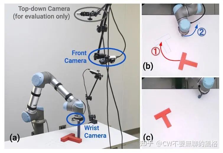
这里以论文中的 demo 为例，这个任务叫 Push-T，顾名思义，就是要让 agent 将一个 T 型的块状物体推至指定的目标区域。具体是使用一个圆形末端执行器将一个 T 型块推到 T 型目标区域，最佳情况是使 T 型块与 T 型区域完全重合。通过对 T 型块和末端执行器设置随机初始条件(例如位置、角度、速度等物理条件)来增加任务的变数(variation)，以考验 agent 的能力。

此外，论文中提到这个任务有两个版本，其中一个是没有观测图像作为条件的，取而代之的是以 T 型块的位置和角度作为条件，我们这里的 demo 是以观测图像为条件的版本。

环境(Env)

先来构建物理环境，主要以继承 gym.Env(https:///www.gymlibrary.dev/api/core/) 类来实现。

class PushTImgEnv(gym.Env):
    # 定义与环境相关的元数据，包括：
    # 1. 渲染模式 `render.modes`
    # 2. 帧率 `video.frames_per_second`
    metadata = {
        # 'rgb_array' 代表以 RGB 数组的形式渲染环境，通常用于模型的输入
        'render.modes': ['rgb_array'],
        'video.frames_per_second': 10
    }

    def __init__(
        self,
        legacy=False,
        block_cog=None,
        damping=None,
        render_size=96,
        render_action=False,
        reset_to_state=None
    ):
        # 是否兼容旧版本
        self.legacy = legacy

        # 设置随机种子
        self._seed = None
        self.seed()

        # 模拟频率，即物理仿真每秒钟执行多少步
        # 其倒数是时间间隔 dt，因此 `sim_hz` 越大 dt 越小，模拟效果越平滑和精细
        # 这里是每秒仿真100次物理引擎(pymunk)
        self.sim_hz = 100
        # 控制频率，表示智能体每秒执行多少次决策（即每秒采取多少次动作）
        # sim_hz / control_hz 代表 agent 的一次决策会由物理环境分多少步来完成
        self.control_hz = self.metadata['video.frames_per_second']

        # 比例-微分控制器 PD-Control 的比例(`k_p`)和微分(`k_v`)系数，用于控制 agent 的运动，
        # 前者越大，agent 越快靠近目标；后者越大，阻尼越强，防止 agent 冲过目标点
        self.k_p, self.k_v = 100, 20

        # pygame 窗口大小
        self.window_size = ws = 512
        # 渲染图像大小
        self.render_size = render_size
        # 是否渲染动作
        self.render_action = render_action

        # 观测状态空间：包括观测图像和 agent 所在位置
        self.observation_space = spaces.Dict({
            'image': spaces.Box(
                low=0., high=1.,
                shape=(3, render_size, render_size),
                dtype=np.float32
            ),
            'agent_pos': spaces.Box(
                low=0., high=ws,
                shape=(2,), dtype=np.float32
            )
        })

        # 动作空间：代理的目标位置
        self.action_space = spaces.Box(
            np.array([0, 0], dtype=np.float64),
            np.array([ws, ws], dtype=np.float64),
            shape=(2,),
            dtype=np.float64
        )

        # 质心, ‘cog' 是 'center of gravity' 的缩写
        self.block_cog = block_cog
        # 与摩擦力相关的阻尼系数
        self.damping = damping

        # 存储 pymunk 物理空间的实例
        # 它管理所有物理对象(如刚体、形状、关节等)以及它们之间的交互
        self.space = None

        # 最近一次执行的动作
        self.latest_action = None

        # 重置时恢复的状态
        self.reset_to_state = reset_to_state

        self.render_cache = None

    def seed(self, seed: int = None):
        # 若未指定随机种子数，则随机设一个
        if seed isNone:
            seed = np.random.randint(0, 25536)

        # 将随机种子值和numpy的随机生成器设置到属性中
        self._seed = seed
        self.np_random = np.random.default_rng(seed=seed)

通过以上代码可以看到，观测状态包括图像和 agent 位置，前者是 (3, H, W) 的 shape，值域归一化至 [0, 1]；而agent 位置的 shape 是 (2,)，代表 x, y 坐标，值域是 [0, ws]，ws 相当于“地图大小”。 至于动作空间 action_space，它实际上代表 agent 的目标位置， 也是 x, y 二维坐标，每个维度的值域都是 [0, ws]。

以上是类的初始化方法，现在来看看物理环境具体是如何搭起来的：

    def _setup(self):
        # 实例化 Pymunk 空间对象
        self.space = pymunk.Space()
        # 设置重力
        # 重力是一个二维向量，通常表示为 (x, y)，
        # 其中 x 和 y 分别表示重力在水平方向和垂直方向上的分量
        self.space.gravity = 0, 0
        # 设置阻尼系数
        # 设置为0表示没有外力作用的情况下不会减速
        self.space.damping = 0

        # 添加墙壁，通过添加线段来围成封闭区域
        # `add_segment` 代表在两点之间连接线段，点坐标是(x,y)形式，以下线段粗细(半径)都是2
        walls = [
            self._add_segment((5, 506), (5, 5), 2),
            self._add_segment((5, 5), (506, 5), 2),
            self._add_segment((506, 5), (506, 506), 2),
            self._add_segment((506, 506), (5, 506), 2)
        ]
        self.space.add(*walls)

        # 实例化代理对象，添加到物理空间中
        # 设置代理对象为一个圆，指定了位置(x,y)和半径
        self.agent = self.add_circle(pos=(256, 400), radius=15)
        # 实例化T型块，添加到物理空间中，
        # 指定了位置(x,y)和角度
        self.block = self.add_tee(pos=(256, 300), angle=0)
        # 设置目标区域的位置和角度
        self.goal_pose = np.array([256, 256, np.pi / 4])
        # 设置目标区域的颜色
        self.goal_color = pygame.Color('LightGreen')

        # 在物理空间中注册一个碰撞处理器，专门处理所有碰撞类型为 0 的物体之间的碰撞事件
        # 在 pymunk 里，每种形状的物体都有一个 `collision_type` 属性，默认是 0，
        # 由于这里没有对各形状物体的碰撞类型进行设置，因此会检测所有物体之间的碰撞
        self.collision_handler = self.space.add_collision_handler(0, 0)
        # 设置碰撞处理器的回调函数
        self.collision_handler_post_solve = self._handle_collision
        # 环境中发生碰撞接触的点数，初始为0
        self.n_contact_points = 0

        # 设置环境的最大得分
        self.max_score = 50 * 100
        # 设置成功完成任务的阀值
        # 即T型块的位置与目标区域有95%的重叠即算成功完成任务
        self.success_threshold = 0.95

接着进一步看看向物理环境中添加墙壁(_add_segment)、agent 末端执行器(add_circle) 以及 T 型块(add_tee)具体是如何实现的：

    def _add_segment(
        self,
        p1: Tuple[float, float],
        p2: Tuple[float, float],
        r: float,
        color: str = 'LightGray'
    ):
        shape = pymunk.Segment(
            self.space.static_body,  # 静态(不会移动的)刚体
            p1, p2, r
        )
        shape.color = pygame.Color(color)

        return shape

    def add_circle(
        self,
        pos: Tuple[float, float],
        radius: float,
        friction: float = 1.0,
        color: str = 'RoyalBlue'
    ):
        # 实例化刚体
        # `KINEMATIC` 代表运动学体，不会受物理引擎的力和冲量影响，
        # 即不会被重力、碰撞等自动推动，只能通过手动设置它的位置、速度或角度来移动它
        # 这种设置通常用于末端执行器
        body = pymunk.Body(body_type=pymunk.Body.KINEMATIC)
        body.position = pos
        # 摩擦系数
        body.friction = friction

        # 设置形状，圆心位置在上面已指定
        shape = pymunk.Circle(body, radius)
        shape.color = pygame.Color(color)

        self.space.add(body, shape)

        return body

    def add_tee(
        self,
        pos: Tuple[float, float],
        angle: float,
        friction: float = 1.,
        scale: float = 30.,
        color: str = 'LightSlateGray',
        mask = pymunk.ShapeFilter.ALL_MASKS()  # 参与所有碰撞检测
    ):
        # 质量
        mass = 1
        # 长宽比
        length = 4

        # T型块水平部分矩形的四个顶点
        vertices_horizon = [
            (-length * scale / 2, 0),
            (length * scale / 2, 0),
            (length * scale / 2, scale),
            (-length * scale / 2,  scale)
        ]
        # 设置动量
        inertial1 = pymunk.moment_for_poly(mass, vertices_horizon)

        # T型块竖直部分矩形的四个顶点
        vertices_vertical = [
            (-scale / 2, scale),
            (scale / 2, scale),
            (scale / 2, length * scale),
            (-scale / 2, length * scale)
        ]
        # 设置动量
        inertial2 = pymunk.moment_for_poly(mass, vertices=vertices_vertical)

        # 实例化刚体，动量为两部分之和
        body = pymunk.Body(mass=mass, moment=inertial1 + inertial2)

        # 设置T型块两部分的形状、颜色以及碰撞检测
        shape1 = pymunk.Poly(body, vertices_horizon)
        shape1.color = pygame.Color(color)
        shape1.filter = pymunk.ShapeFilter(mask=mask)

        shape2 = pymunk.Poly(body, vertices_vertical)
        shape2.color =pygame.Color(color)
        shape2.filter = pymunk.ShapeFilter(mask=mask)

        # 设置质心为两部分矩形块质心的均值
        body.center_of_gravity = (
            shape1.center_of_gravity +
            shape2.center_of_gravity
        ) / 2.

        # 设置T型块的位置、角度以及摩擦系数
        body.position = pos
        body.angle = angle
        body.friction = friction

        # 将刚体和形状添加到环境实例中
        self.space.add(body, shape1, shape2)

        return body

    def _handle_collision(self, arbiter: pymunk.Arbiter, *args):
        # PyMunk 的 Arbiter 对象，包含了碰撞事件的所有信息，例如碰撞点、碰撞形状等
        # `contact_point_set.points` 包含了当前碰撞事件中所有碰撞接触点的列表
        self.n_contact_points += len(arbiter.contact_point_set.points)

通常在实例化环境对象后，首先都会调用其 reset() 方法，相当于一种初始化，现在就来看看这其中的逻辑：

    def _get_info(self):
        """
        返回代理位置、代理速度、T型块的姿态位置&角度、目标区域的位置&角度、每步接触点数量
        """

        # 计算 agent 的每个决策实际在物理引擎中运行的步数
        n_steps = self.sim_hz // self.control_hz
        # 计算每步的接触点数量
        n_contact_points_per_step = int(math.ceil(self.n_contact_points / n_steps))

        return {
            'pos_agent': np.array(self.agent.position),
            'vel_agent': np.array(self.agent.velocity),
            'block_pose': np.array(list(self.block.position) + [self.block.angle]),
            'goal_pose': self.goal_pose,
            'n_contacts': n_contact_points_per_step
        }

    def reset(self):
        # 首先调用 `_set_up()` 方法构建物理环境
        self._setup()

        # 设置T型块的质心和环境的阻尼系数(若初始化方法中指定了相关参数)
        if self.block_cog isnotNone:
            self.block.center_of_gravity = self.block_cog
        if self.damping isnotNone:
            self.space.damping = self.damping

        state = self.reset_to_state
        # 若没有指定重置时状态值，则随机设置
        if state isNone:
            rs = np.random.RandomState(seed=self._seed)

            state = [
                # agent 位置
                rs.randint(50, 450), rs.randint(50, 450),
                # T型块位置
                rs.randint(100, 400), rs.randint(100, 400),
                # T型块角度：[-pi, pi]
                (2 * rs.randn() - 1) * np.pi
            ]
        self._set_state(state)

        # 调用 `_get_obs()` 方法获取观测状态
        obs = self._get_obs()
        # 调用 `_get_info()` 方法获取环境信息
        info = self._get_info()

        return obs, info

进一步看看其中的 _set_state() 方法是如何将指定状态 state 设置到 agent 和 T型块并在物理空间中生效的：

    def _set_state(self, state):
        # 将 `state` 装换为列表
        if isinstance(state, np.ndarray):
            state = state.tolist()

        # 对应取出 agent 位置、T型块的位置及角度
        pos_agent = state[:2]
        pos_block = state[2:4]
        rot_block = state[4]

        # 设置 agent 位置
        self.agent.position = pos_agent
        # 设置T型块的角度和位置
        # setting angle rotates with respect to center of mass
        # therefore will modify the geometric position
        # if not the same as CoM
        # therefore should be modified first.
        if self.legacy:
            # 旧版本的设置方式
            self.block.position = pos_block
            self.block.angle = rot_block
        else:
            # 由于设置角度(相对于质心)可能会改变几何中心(如果于质心不一致的话)
            # 因此要先设置角度，最后设置位置
            self.block.angle = rot_block
            self.block.position = pos_block

        # 让环境运行一小步以使得以上设置生效
        # 1.0 / sim_hz = dt
        self.space.step(1.0 / self.sim_hz)

然后再来看看观测状态的获取，其中观测图像的获取需要通过渲染帧来实现：

    def _get_obs(self):
        # 将代理位置转换为 np.array
        agent_pos = np.array(self.agent.position)

        # 获取渲染图像
        img = self._render_frame()
        # 归一化图像至 [0, 1]
        img_obs = img.astype(np.float32) / 255.
        # 将最后一个维度移动至第一维：HWC->CHW
        img_obs = np.moveaxis(img_obs, -1, 0)

        # draw action
        # 在渲染图上画出动作
        if self.latest_action isnotNone:
            action = np.array(self.latest_action)
            # 缩放到渲染图的空间大小
            coord = (action / self.window_size * self.render_size).astype(np.int32)
            marker_size = int(8 / 96 * self.render_size)
            thickness = int(1 / 96 * self.render_size)

            cv2.drawMarker(
                img, coord,
                color=(255, 0, 0),  # bgr 蓝色
                markerType=cv2.MARKER_CROSS,  # 十字形
                markerSize=marker_size,
                thickness=thickness
            )

        self.render_cache = img

        return {
            'image': img_obs,
            'agent_pos': agent_pos
        }

现在来看看渲染相关的实现：

    def  _get_goal_pose_body(
        self,
        pose: np.ndarray,
        mass: float = 1.,
        width: float = 50.,
        height: float = 100.
    ):
        # 根据质量和宽、高计算惯性矩
        inertia = pymunk.moment_for_box(mass, (width, height))
        # 实例化刚体对象
        body = pymunk.Body(mass=mass, moment=inertia)

        # 设置刚体的位置和角度
        # preserving the legacy assignment order for compatibility
        # the order here dosn't matter somehow, maybe because CoM is aligned with body origin
        body.position = pose[:2].tolist()
        body.angle = pose[2]

        return body

    def _render_frame(self):
        # 创建空白画布
        canvas = pygame.Surface((self.window_size,) * 2)
        # 纯白
        canvas.fill((255,) * 3)

        # DrawOptions 是一个自定义类，继承自 pymunk.SpaceDebugDrawOptions，
        # 用于配置如何在 Pygame 窗口中绘制物理空间中的对象
        draw_options = DrawOptions(canvas)

        # 绘制目标区域
        # 调用 `self._get_goal_pose_body()` 获取代表目标区域的刚体
        goal_body = self._get_goal_pose_body(self.goal_pose)
        # 计算T型块顶点在目标区域的坐标
        for shape in self.block.shapes:
            goal_points = [
                # 用于将 Pymunk 物理引擎中的坐标转换为 Pygame 可以理解的屏幕坐标。
                # Pymunk 的坐标系与 Pygame 的坐标系有所不同，Pymunk 的原点在屏幕左下角，
                # 而 Pygame 的原点在屏幕左上角，因此需要进行坐标转换。
                pymunk.pygame_util.to_pygame(
                    # 将物体的局部坐标（相对于物体自身的坐标系）转换为世界坐标（全局坐标系）
                    goal_body.local_to_world(v),
                    draw_options.surface
                ) for v in shape.get_vertices()  # 这些顶点是相对于形状所在刚体的局部坐标
            ]
            # 将目标区域的顶点绘制到画布上
            pygame.draw.polygon(canvas, self.goal_color, goal_points)

        # Draw agent and block.
        # 将物理空间中的所有对象（包括 agent 和 block）绘制到 Pygame 的画布上。
        # 这些对象的绘制方式会根据 draw_options 中的配置来决定
        self.space.debug_draw(draw_options)

        # 将画布转换成 numpy array 图像并缩放到渲染窗口大小(`self.render_size`)
        # (w, h, c) -> (h, w, c)
        img = np.transpose(
            # `pygame.surfarray.pixels3d()` 获取一个 Surface 对象的像素数据。
            # 它返回一个三维 NumPy 数组，数组的形状为 (width, height,channels)
            np.array(pygame.surfarray.pixels3d(canvas)),
            axes=(1, 0, 2)
        )
        img = cv2.resize(img, (self.render_size,) * 2)

        return img

    def render(self):
        if self.render_cache isNone:
            self._get_obs()

        return self.render_cache

由此可知，目标区域的 T 型块是仅在渲染的时候才通过 _get_goal_pose_body() 方法实例化出来的。下面展示出用于在 pygame 中实现绘制的 DrawOptions 类及相关逻辑实现：

positive_y_is_up: bool = False
"""Make increasing values of y point upwards.

When True::

    y
    ^
    |      . (3, 3)
    |
    |   . (2, 2)
    |
    +------ > x

When False::

    +------ > x
    |
    |   . (2, 2)
    |
    |      . (3, 3)
    v
    y

"""

def to_pygame(p: Tuple[float, float], surface: pygame.Surface) -> Tuple[int, int]:
    """Convenience method to convert pymunk coordinates to pygame surface
    local coordinates.

    Note that in case positive_y_is_up is False, this function wont actually do
    anything except converting the point to integers.
    """

    if positive_y_is_up:
        return round(p[0]), surface.get_height() - round(p[1])
    else:
        return round(p[0]), round(p[1])

def light_color(color: SpaceDebugColor):
    color = np.minimum(
        1.2 * np.float32([color.r, color.g, color.b, color.a]),
        np.float32([255])
    )
    color = SpaceDebugColor(r=color[0], g=color[1], b=color[2], a=color[3])

    return color

class DrawOptions(pymunk.SpaceDebugDrawOptions):
    def __init__(self, surface: pygame.Surface) -> None:
        """Draw a pymunk.Space on a pygame.Surface object.

        Typical usage::

        >>> import pymunk
        >>> surface = pygame.Surface((10,10))
        >>> space = pymunk.Space()
        >>> options = pymunk.pygame_util.DrawOptions(surface)
        >>> space.debug_draw(options)

        You can control the color of a shape by setting shape.color to the color
        you want it drawn in::

        >>> c = pymunk.Circle(None, 10)
        >>> c.color = pygame.Color("pink")

        See pygame_util.demo.py for a full example

        Since pygame uses a coordiante system where y points down (in contrast
        to many other cases), you either have to make the physics simulation
        with Pymunk also behave in that way, or flip everything when you draw.

        The easiest is probably to just make the simulation behave the same
        way as Pygame does. In that way all coordinates used are in the same
        orientation and easy to reason about::

        >>> space = pymunk.Space()
        >>> space.gravity = (0, -1000)
        >>> body = pymunk.Body()
        >>> body.position = (0, 0) # will be positioned in the top left corner
        >>> space.debug_draw(options)

        To flip the drawing its possible to set the module property
        :py:data:`positive_y_is_up` to True. Then the pygame drawing will flip
        the simulation upside down before drawing::

        >>> positive_y_is_up = True
        >>> body = pymunk.Body()
        >>> body.position = (0, 0)
        >>> # Body will be position in bottom left corner

        :Parameters:
                surface : pygame.Surface
                    Surface that the objects will be drawn on
        """

        self.surface = surface
        super(DrawOptions, self).__init__()

    def draw_circle(
        self,
        pos: Vec2d,
        angle: float,
        radius: float,
        outline_color: SpaceDebugColor,  # 边缘颜色
        fill_color: SpaceDebugColor,  # 填充颜色
    ) -> None:
        # 圆心位置
        p = to_pygame(pos, self.surface)

        # 绘制圆
        # 0 表示填充，1表示绘制边缘
        pygame.draw.circle(
            self.surface,
            # 填充颜色
            fill_color.as_int(),
            p, round(radius), 0
        )
        # 绘制内圆
        pygame.draw.circle(
            self.surface,
            light_color(fill_color).as_int(),
            p, round(radius - 4), 0
        )

        # 圆上的边缘点
        circle_edge = pos + Vec2d(radius, 0).rotated(angle)
        p2 = to_pygame(circle_edge, self.surface)

        # 根据圆的半径设定线条粗细
        line_r = 2if radius > 20else1
        # pygame.draw.lines(self.surface, outline_color.as_int(), False, [p, p2], line_r)

    def draw_segment(self, a: Vec2d, b: Vec2d, color: SpaceDebugColor) -> None:
        p1 = to_pygame(a, self.surface)
        p2 = to_pygame(b, self.surface)

        # False 代表不闭合线段，即不绘制多边形
        pygame.draw.aalines(self.surface, color.as_int(), False, [p1, p2])

    def draw_fat_segment(
        self,
        a: Tuple[float, float],
        b: Tuple[float, float],
        radius: float,
        outline_color: SpaceDebugColor,
        fill_color: SpaceDebugColor,
    ) -> None:
        p1 = to_pygame(a, self.surface)
        p2 = to_pygame(b, self.surface)

        r = round(max(1, radius * 2))
        # `r` 代表线段宽度的半径
        pygame.draw.lines(self.surface, fill_color.as_int(), False, [p1, p2], r)

        if r > 2:
            # 计算法向量
            orthog = [abs(p2[1] - p1[1]), abs(p2[0] - p1[0])]
            if orthog[0] == 0and orthog[1] == 0:
                return

            # 对法向量缩放，使其长度等于半径
            scale = radius / (orthog[0] * orthog[0] + orthog[1] * orthog[1]) ** 0.5
            orthog[0] = round(orthog[0] * scale)
            orthog[1] = round(orthog[1] * scale)
            # 设置矩形的四个顶点，每对顶点沿法向量方向穿过线段的其中一个顶点，
            # 并且这对顶点之间的长度等于线段的宽度(2 * r)
            points = [
                (p1[0] - orthog[0], p1[1] - orthog[1]),
                (p1[0] + orthog[0], p1[1] + orthog[1]),
                (p2[0] + orthog[0], p2[1] + orthog[1]),
                (p2[0] - orthog[0], p2[1] - orthog[1]),
            ]
            # 以绘制矩形的方式来表示粗线段
            pygame.draw.polygon(self.surface, fill_color.as_int(), points)

            # 将线段的两个端点绘作圆
            pygame.draw.circle(
                self.surface,
                fill_color.as_int(),
                (round(p1[0]), round(p1[1])),
                round(radius),
            )
            pygame.draw.circle(
                self.surface,
                fill_color.as_int(),
                (round(p2[0]), round(p2[1])),
                round(radius),
            )

    def draw_polygon(
        self,
        verts: Sequence[Tuple[float, float]],
        radius: float,
        outline_color: SpaceDebugColor,
        fill_color: SpaceDebugColor,
    ) -> None:
        ps = [to_pygame(v, self.surface) for v in verts]
        # 添加上第一个顶点形成封闭区域
        ps += [ps[0]]
        pygame.draw.polygon(self.surface, light_color(fill_color).as_int(), ps)

        radius = 2
        if radius > 0:
            # 在顶点之间绘制粗线段
            for i in range(len(verts)):
                a = verts[i]
                b = verts[(i + 1) % len(verts)]
                self.draw_fat_segment(a, b, radius, fill_color, fill_color)

    def draw_dot(
        self, size: float,
        pos: Tuple[float, float],
        color: SpaceDebugColor
    ) -> None:
        p = to_pygame(pos, self.surface)
        # 0代表填充，1代表绘制边缘
        pygame.draw.circle(self.surface, color.as_int(), p, round(size), 0)

由以上可知，在 pygame 中，默认情况下 y 坐标是越大越往下的，也就是原点在左上方。

最后来看看在 agent 做出决策(生成了目标动作)并在环境中执行后具体会发生哪些事情：

    def step(self, action: np.ndarray):
        # 时间微分 dt
        dt = 1. / self.sim_hz
        # 一次决策(动作)在物理引擎中执行的步数
        n_steps = self.sim_hz // self.control_hz

        # 重置碰撞接触点数量
        self.n_contact_points = 0

        if action isnotNone:
            # 记录最新一次的动作
            self.latest_action = action

            # 将 agent 的一次决策分成多步物理仿真细致执行，
            # 每一步都用 PD(比例-微分) 控制器调整 agent 的速度，并推进物理引擎一步，以实现平滑、真实的物理运动。
            for _ in range(n_steps):
                # Step PD control.
                # action - self.agent.position 代表目标位置与当前位置的距离，越远则加速度越大，希望尽快接近目标位置
                # Vec2d(0, 0) - self.agent.velocity 代表目标速度与当前速度之差，目标速度是0是因为希望 agent 在目标位置停下来，
                # 防止冲过头，这部分起到“反向加速度”的作用。
                acceleration = self.k_p * (action - self.agent.position) + \
                    self.k_v * (Vec2d(0, 0) - self.agent.velocity)
                # 欧拉法则
                self.agent.velocity += acceleration * dt
                # Step physics.
                self.space.step(dt)

        # 根据目标区域的位置获取刚体
        goal_body = self._get_goal_pose_body(self.goal_pose)
        # 获取目标T型区域与当前 T 型块的多边形形状，以便后续计算两者的重叠面积
        goal_geom = pymunk_to_shapely(goal_body, self.block.shapes)
        block_geom = pymunk_to_shapely(self.block, self.block.shapes)

        # 根据T型块与目标区域的重叠面积计算奖励
        intersection = goal_geom.intersection(block_geom).area
        # 重叠面积占目标区域的大小
        coverage = intersection / goal_geom.area
        # 根据阀值(`success_threshold`)对奖励值进行缩放
        reward = np.clip(coverage / self.success_threshold, 0., 1.)

        # 若T型块覆盖目标区域的面积超过阀值则表示任务成功完成
        done = coverage > self.success_threshold
        # 设置终止和截断信号
        # 通常 `terminated` 代表成功/失败导致任务结束；
        # 而 `truncated` 是指达到最大交互次数的限制而终止任务。
        # 但这里不作区分，将两者等价
        terminated = truncated = done

        # 获取观测值和环境信息
        obs = self._get_obs()
        info = self._get_info()

        return obs, reward, terminated, truncated, info

其中 pymunk_to_shapely() 是类之外的通用方法，用于将 pymunk 的刚体形状转换为 shapely 的几何多边形以方便计算面积：

def pymunk_to_shapely(body, shapes):
    """
    将 Pymunk形状转换为 Shapely多边形。

    参数:
    - body: Pymunk 刚体对象，用于将局部坐标转换为世界坐标。
    - shapes: Pymunk 形状列表，包含要转换的形状。

    返回:
    - sg.MultiPolygon: 一个 Shapely 多边形对象，包含所有转换后的形状。
    """

    # 初始化一个空列表，用于存储转换后的 Shapely多边形
    geoms = list()
    # 遍历给定的 Pymunk 形状列表
    for shape in shapes:
        if isinstance(shape, pymunk.shapes.Poly):
            # 将多边形的顶点从局部坐标转换为世界坐标
            verts = [body.local_to_world(v) for v in shape.get_vertices()]
            # 将第一个顶点添加到最后，以形成闭合的多边形
            verts += [verts[0]]
            geoms.append(sg.Polygon(verts))
        else:
            raise RuntimeError(f'Unsupported shape type {type(shape)}')

    return sg.MultiPolygon(geoms) 

OK，让我们实例化这个环境对象来测试并输出一些信息来看看：

# 0. create env object
env = PushTImageEnv()

# 1. seed env for initial state.
# Seed 0-200 are used for the demonstration dataset.
env.seed(1000)

# 2. must reset before use
env.reset()

# 3. 2D positional action space [0,512]
action = env.action_space.sample()

# 4. Standard gym step method
obs, reward, terminated, truncated, info = env.step(action)

# prints and explains each dimension of the observation and action vectors
with np.printoptions(precision=4, suppress=True, threshold=5):
    print(
        f"obs['image'].shape: {obs['image'].shape}, "
        f"dtype: {obs['image'].dtype}, range: [0, 1]"
    )
    print(
        f"obs['agent_pos'].shape: {obs['agent_pos'].shape}, "
        f"dtype: {obs['agent_pos'].dtype}, range: [0, {env.window_size}]"
    )
    print(
        f"action.shape: {action.shape}, "
        f"dtype: {action.dtype}, range: [0, {env.window_size}]"
    )

print(f"reward: {reward}")
print(terminated, truncated)
print(f"info: {info}")
print(f"action: {action}")

如果没毛病，将会得到以下输出：

obs['image'].shape: (3, 96, 96), dtype: float32, range: [0, 1]
obs['agent_pos'].shape: (2,), dtype: float64, range: [0, 512]
action.shape: (2,), dtype: float64, range: [0, 512]

reward: 0.18776528434724993
False False
info: {'pos_agent': array([123.35925412, 181.11840283]), 'vel_agent': array([-172.61211042,  760.74757759]), 'block_pose': array([292.        , 351.        ,  -9.64681177]), 'goal_pose': array([256.        , 256.        ,   0.78539816]), 'n_contacts': 0}
action: [ 90.86524338 324.3281689 ]

数据集

以上构建的环境主要用在推理期间进行测试，而模型训练还是需要在数据集上来完成。假设我们已经采集了一批数据样本并存储至某个指定路径，每个样本包括当前时间步的观测图像、agent 位置 以及目标动作(注意不是序列，是单步动作)，现在就来构建这个数据集的类，它继承自 Pytorch 的 Dataset 类：

def get_data_stats(data):
    data = data.reshape(-1, data.shape[-1])

    return {
        'min': np.min(data, axis=0),
        'max': np.max(data, axis=0)
    }

def normalize_data(data, stats):
    # nomalize to [0,1]
    normalized = (data - stats['min']) / (stats['max'] - stats['min'])
    # [0,1] -> [-1,1]
    normalized = 2 * normalized - 1

    return normalized

class PushTImageDataset(torch.utils.data.Dataset):
    def __init__(
        self,
        dataset_path: str,
        pred_horizon: int,
        obs_horizon: int,
        action_horizon: int
    ):
        # read from zarr dataset
        dataset_root = zarr.open(dataset_path, mode="r")

        # float32, [0,1], (N,96,96,3)
        train_image_data = dataset_root["data"]["img"][:]
        # (N,H,W,C) -> (N,C,H,W)
        train_image_data = np.moveaxis(train_image_data, -1, 1)

        # agent 位置、目标动作
        train_data = {
            # first two dims of state vector are agent (i.e. gripper) locations
            "agent_pos": dataset_root["data"]["state"][:, :2],
            "action": dataset_root["data"]["action"][:]
        }

        # episode
        episode_ends = dataset_root["meta"]["episode_ends"][:]

        # compute start and end of each state-action sequence
        # also handles padding
        # 计算每个状态-动作序列的起止索引(考虑了 padding 的情况)
        indices = create_sample_indices(
            episode_ends=episode_ends,
            sequence_length=pred_horizon,
            pad_before=obs_horizon - 1,
            pad_after=action_horizon - 1
        )

        # compute statistics and normalized data to [-1,1]
        stats = {}
        normalized_train_data = {}
        for key, data in train_data.items():
            # 计算数据每个维度的最大最小值，用于归一化
            stats[key] = get_data_stats(data)
            # 利用最大最小值进行归一化
            normalized_train_data[key] = normalize_data(data, stats[key])
        # images are already normalized
        normalized_train_data['image'] = train_image_data

        self.stats = stats
        self.indices = indices
        self.normalized_train_data = normalized_train_data

        # 观测状态的范围(即每次 agent 以多少步的状态作为观测条件)，当前时间步加上以往时间步的数量
        self.obs_horizon = obs_horizon
        # 预测多少步动作，由第一个观测状态开始(而不是当前时间步)
        self.pred_horizon = pred_horizon
        # 实际执行多少步动作，当前时间步开始，加上未来时间步的数量
        self.action_horizon = action_horizon

    def __len__(self):
        return len(self.indices) 

注意，由于收集的每个数据样本都是单步的状态和动作，因此我们需要自行构建起序列，以适配 diffusion policy 的玩法，最终将每个状态-动作序列作为训练样本。每个序列都需要指定起止样本索引，这样才能够从数据集中取出序列所包含的样本点，而为序列设置样本索引的逻辑就在以上的 create_sample_indices() 方法中，序列长度等于预测范围 pred_horizon，也就是在模型每次生成的动作序列中包含多少步动作。

与此同时，还有观测范围 obs_horizon 和 动作范围action_horizon 的存在，前者指的是 agent 每次决策前要结合多少步的观测状态，它是 “向前看” 的，也就是只能获取当前时间与过去的状态；后者代表 agent 生成一个动作序列后，实际执行了其中的多少步，它是“向后走” 的，即只能由当下开始执行逐渐走向未来(周董：想回到过去~)。哦，对了，模型预测的 pred_horizon 则是同时包含过去和未来的，也就是它需要覆盖 obs_horizon 以及 action_horizon 的范围，即有以下关系：

pred_horizon = obs_horizon + action_horizon

由于原始数据是分为多个 episode 的(即回合制)，每个 episode 要保持彼此独立，因此还要保证构建的序列不能够“跨回合”，也就是确保序列中的每个数据点是位于同一个 episode 中的。然而，以上这种“向前看”和“向后走”的机制，就有可能导致我们构建的序列会超出其本应所在的 episode，比如位于某个 episode 起始的数据点，由于“向前看”的机制，因此不小心搂到了前一个 episode 的妹子(哎哟，这可就出大事了..)；而位于 episode 末尾的数据点，由于“向后走”的机制，因此也会牵到下一个 episode 的哥们儿(嫌弃脸 -_-||)。

为了避免以上事故发生，老练的炼丹师们自然就想到用 padding 的套路去解决啦！在从数据集中采集数据点而构建序列时，若发现“向前看”会跨到前一个 episode 的情况，则在数据点的前面进行 padding；同理，若发现“向后走”会走到下一个 episode，那么就在数据点的后面进行 padding。

现在让我们一起来看看以上所提到的具体实现：

def create_sample_indices(
    episode_ends: np.ndarray,
    sequence_length: int,
    pad_before: int = 0, pad_after: int = 0
):
    indices = []

    # 依次在每个 episode 中计算所有可能的序列起止索引
    # 序列长度由预测范围(`pred_horizon`)决定
    for i, end_idx in enumerate(episode_ends):
        # 每个回合的起始索引
        start_idx = episode_ends[i - 1] if i else0
        # 每个回合的长度(包含多少个时间步)
        episode_length = end_idx - start_idx

        # 在本 episode 内相对于 `start_idx` 来说的最小、最大起始索引
        # 负数代表在 `start_idx` 之前, pad_before 由观测范围(`obs_horizon`)决定
        min_start_idx = -pad_before
        # 要避免超出当前所 episode 位置(考虑了 padding)，所以有最大限制，pad 由动作执行范围(`action_horizon`)决定
        max_start_idx = episode_length - sequence_length + pad_after

        # 在 episode 内采样数据
        # 根据起始索引在当前 episode 一次采样多个序列
        for idx in range(min_start_idx, max_start_idx + 1):
            # `buffer_start_idx`, `buffer_end_idx` 用于在数据集中取出样本点序列(然后可能进行 padding)
            buffer_start_idx = max(0, idx) + start_idx
            buffer_end_idx = min(idx + sequence_length, episode_length) + start_idx

            # 头部 padding 的长度，当观测范围超出当前 episode 起始时(此时 `idx` 为负数)，需要 padding
            start_offset = max(-idx, 0)
            # 尾部 padding 的长度，若超出当前 episode 的结尾，则需要 padding
            end_offset = max(idx + sequence_length - episode_length, 0)

            # 在对 buffer 进行 padding 后，标记真实样本(非 padding)在 buffer 中的位置，
            # buffer 代表一个样本序列，长度为 `sequence_length`
            # buffer[sample_start_idx:sample_end_idx]就代表真实而非 padding 的数据样本
            sample_start_idx = start_offset
            sample_end_idx = sequence_length - end_offset

            indices.append([
                buffer_start_idx, buffer_end_idx,
                sample_start_idx, sample_end_idx
            ])

    return np.array(indices)

def sample_sequence(
    train_data: Dict, sequence_length: int,
    buffer_start_idx: int, buffer_end_idx: int,
    sample_start_idx: int, sample_end_idx: int
):
    result = {}
    for key, input_arr in train_data.items():
        # 根据 `buffer_start_idx`, 'buffer_end_idx` 从数据集中取出样本
        sample = input_arr[buffer_start_idx:buffer_end_idx]
        data = sample

        # 判断是否有 padding
        if sample_start_idx > 0or sample_end_idx < sequence_length:
            # 初始化序列数据
            data = np.zeros(
                (sequence_length, *input_arr.shape[1:]),
                dtype=input_arr.dtype
            )

            if sample_start_idx > 0:
                # 设置头部填充的都是第一个样本
                data[:sample_start_idx] = sample[0]
            if sample_end_idx < sequence_length:
                # 设置尾部填充的都是最后一个样本
                data[sample_end_idx:] = sample[-1]

            # 将真实样本放置到对应位置
            data[sample_start_idx:sample_end_idx] = sample

        result[key] = data

    return result

最终，再利用 PushTImageDataset 的 __getitem__() 方法取出样本，每个样本就是一个序列，传入这个方法的 idx 索引对应以上构建好的序列索引集合(self.indices) ，而非原数据集中每个数据点的索引。

    def __getitem__(self, idx):
        # get the start/end indices for this datapoint
        buffer_start_idx, buffer_end_idx, \
            sample_start_idx, sample_end_idx = self.indices[idx]

        # get nomralized data using these indices
        samples = sample_sequence(
            self.normalized_train_data,
            self.pred_horizon,
            buffer_start_idx, buffer_end_idx,
            sample_start_idx, sample_end_idx
        )

        # 每个时刻只能观测到当前及之前的状态
        # discard unused observations
        samples['image'] = samples['image'][:self.obs_horizon]
        samples['agent_pos'] = samples['agent_pos'][:self.obs_horizon]

        return samples

OK，与前面类似，现在也可以实例化一下这个数据集对象并输出一些信息进行测试。作者很贴心地给出了他收集好的数据地址，并且让大家随意下载，感谢真主~ 或者，你也可以上 HuggingFace 整一份：https://huggingface.co/datasets/lerobot/pusht

# download demonstration data from Google Drive
dataset_path = "pusht_cchi_v7_replay.zarr.zip"
ifnot os.path.isfile(dataset_path):
    id = "1KY1InLurpMvJDRb14L9NlXT_fEsCvVUq&confirm=t"
    gdown.download(id=id, output=dataset_path, quiet=False)

# parameters
pred_horizon = 16
obs_horizon = 2
action_horizon = 8
#|o|o|                             observations: 2
#| |a|a|a|a|a|a|a|a|               actions executed: 8
#|p|p|p|p|p|p|p|p|p|p|p|p|p|p|p|p| actions predicted: 16

# create dataset from file
dataset = PushTImageDataset(
    dataset_path,
    pred_horizon,
    obs_horizon,
    action_horizon
)

# create dataloader
dataloader = torch.utils.data.DataLoader(
    dataset,
    batch_size=64, shuffle=True,
    num_workers=os.cpu_count(),
    # accelerate cpu-gpu transfer
    pin_memory=True,
    # don't kill worker process afte each epoch
    persistent_workers=True
)

# visualize data in batch
batch = next(iter(dataloader))
print(f"batch['image'].shape: {batch['image'].shape}")
print(f"batch['agent_pos'].shape: {batch['agent_pos'].shape}")
print(f"batch['action'].shape: {batch['action'].shape}")

# save training data statistics (min, max) for each dim
stats = dataset.stats
for k, v in stats.items():
    print(f"{k}: {v}")

若顺利的话，将得到以下输出：

Downloading...
From: https://drive.google.com/uc?id=1KY1InLurpMvJDRb14L9NlXT_fEsCvVUq&confirm=t
To: /content/pusht_cchi_v7_replay.zarr.zip
100%|██████████| 31.1M/31.1M [00:00<00:00, 115MB/s] 

batch['image'].shape: torch.Size([64, 2, 3, 96, 96])
batch['agent_pos'].shape: torch.Size([64, 2, 2])
batch['action'].shape: torch.Size([64, 16, 2])

agent_pos: {'min': array([13.456424, 32.938293], dtype=float32), 'max': array([496.14618, 510.9579 ], dtype=float32)}
action: {'min': array([12., 25.], dtype=float32), 'max': array([511., 511.], dtype=float32)}

扩散模型

扩散模型的实现没有什么可说的，这里以 U-Net 架构为例，接收 1D 形式的序列输入。哦，对于扩散时间步 timestep(是扩散模型中与噪声强度相关的那个时间步，不是前面物理意义上的时间步)，这里用正弦位置编码的方式(SinusoidalPosEmb)将其编码为 embedding 注入到扩散模型中，然后会和观测条件向量 concat 在一起。

#@markdown ### **Network**
#@markdown
#@markdown Defines a 1D UNet architecture `ConditionalUnet1D`
#@markdown as the noies prediction network
#@markdown
#@markdown Components
#@markdown - `SinusoidalPosEmb` Positional encoding for the diffusion iteration k
#@markdown - `Downsample1d` Strided convolution to reduce temporal resolution
#@markdown - `Upsample1d` Transposed convolution to increase temporal resolution
#@markdown - `Conv1dBlock` Conv1d --> GroupNorm --> Mish
#@markdown - `ConditionalResidualBlock1D` Takes two inputs `x` and `cond`. \
#@markdown `x` is passed through 2 `Conv1dBlock` stacked together with residual connection.
#@markdown `cond` is applied to `x` with [FiLM](https://arxiv.org/abs/1709.07871) conditioning.

class SinusoidalPosEmb(nn.Module):
    def __init__(self, dim):
        super().__init__()
        self.dim = dim

    def forward(self, x):
        device = x.device

        half_dim = self.dim // 2
        emb = torch.exp(
            torch.arange(half_dim, device=device) / (half_dim - 1) *
            -math.log(10000)
        )

        emb = x[:, None] * emb[None, :]
        emb = torch.cat([emb.sin(), emb.cos()], dim=1)

        return emb

class Downsample1d(nn.Module):
    def __init__(self, dim):
        super().__init__()
        self.conv = nn.Conv1d(dim, dim, 3, stride=2, padding=1)

    def forward(self, x):
        return self.conv(x)

class Upsample1d(nn.Module):
    def __init__(self, dim):
        super().__init__()
        self.conv = nn.ConvTranspose1d(dim, dim, 4, stride=2, padding=1)

    def forward(self, x):
        return self.conv(x)

class Conv1dBlock(nn.Module):
    """
        Conv1d --> GroupNorm --> Mish
    """

    def __init__(self, in_channels, out_channels, kernel_size, n_groups=8):
        super().__init__()

        self.block = nn.Sequential(
            nn.Conv1d(
                in_channels, out_channels,
                kernel_size, padding=kernel_size // 2
            ),
            nn.GroupNorm(n_groups, out_channels),
            nn.Mish()
        )

    def forward(self, x):
        return self.block(x)

class ConditionalResidualBlock1d(nn.Module):
    def __init__(
        self,
        in_channels, out_channels,
        cond_dim, kernel_size=3, n_groups=8
    ):
        super().__init__()

        self.out_channels = out_channels
        self.blocks = nn.ModuleList([
            Conv1dBlock(in_channels, out_channels, kernel_size, n_groups=n_groups),
            Conv1dBlock(out_channels, out_channels, kernel_size, n_groups=n_groups)
        ])

        cond_channels = out_channels * 2
        self.cond_encoder = nn.Sequential(
            nn.Mish(),
            nn.Linear(cond_dim, cond_channels),
            nn.Unflatten(-1, (-1, 1))
        )

        self.residual_conv = nn.Conv1d(in_channels, out_channels, 1) \
            if in_channels != out_channels else nn.Identity()

    def forward(self, x, cond):
        """
        params:
            x : [ batch_size x in_channels x horizon ]
            cond : [ batch_size x cond_dim]

        returns:
            out : [ batch_size x out_channels x horizon ]
        """

        out = self.blocks[0](x)

        # (b,d)->(b,2*c,1)
        embed = self.cond_encoder(cond)
        scale, shift = torch.chunk(embed, 2, dim=1)
        # FiLM
        out = scale * out + shift

        out = self.blocks[1](out)
        out = out + self.residual_conv(x)

        return out

class ConditionalUnet1d(nn.Module):
    def __init__(
        self,
        input_dim,
        global_cond_dim,
        diffusion_step_embed_dim=256,
        down_dims=[256, 512, 1024],
        kernel_size=5, n_groups=8
    ):
        """
            input_dim:  Dim of actions.
            global_cond_dim: Dim of global conditioning applied with FiLM
                             in addition to diffusion step embedding.
                             This is usually obs_horizon * obs_dim
            diffusion_step_embed_dim: Size of positional encoding for
                                      diffusion iteration k
            down_dims: Channel size for each UNet level.
                       The length of this array determines numebr of levels.
            kernel_size: Conv kernel size
            n_groups: Number of groups for GroupNorm
        """

        super().__init__()

        # Encode diffusion step
        dsed = diffusion_step_embed_dim
        self.diffusion_step_encoder = nn.Sequential(
            SinusoidalPosEmb(dsed),
            nn.Linear(dsed, dsed * 4),
            nn.Mish(),
            nn.Linear(dsed * 4, dsed)
        )

        cond_dim = dsed + global_cond_dim

        all_dims = [input_dim] + list(down_dims)
        in_out = list(zip(all_dims[:-1], all_dims[1:]))

        # Downblocks
        down_modules = nn.ModuleList()
        for ind, (dim_in, dim_out) in enumerate(in_out):
            is_last = ind == len(in_out) - 1

            down_modules.append(
                nn.ModuleList([
                    ConditionalResidualBlock1d(
                        dim_in, dim_out, cond_dim,
                        kernel_size=kernel_size, n_groups=n_groups
                    ),
                    ConditionalResidualBlock1d(
                        dim_out, dim_out, cond_dim,
                        kernel_size=kernel_size, n_groups=n_groups
                    ),
                    Downsample1d(dim_out) ifnot is_last else nn.Identity()
                ])
            )
        self.down_modules = down_modules

        # MidbLocks
        mid_dim = all_dims[-1]
        self.mid_modules = nn.ModuleList([
            ConditionalResidualBlock1d(
                mid_dim, mid_dim, cond_dim,
                kernel_size=kernel_size, n_groups=n_groups
            ),
            ConditionalResidualBlock1d(
                mid_dim, mid_dim, cond_dim,
                kernel_size=kernel_size, n_groups=n_groups
            )
        ])

        up_modules = nn.ModuleList()
        for dim_in, dim_out in reversed(in_out[1:]):
            up_modules.append(
                nn.ModuleList([
                    ConditionalResidualBlock1d(
                        2 * dim_out, dim_in, cond_dim,
                        kernel_size=kernel_size, n_groups=n_groups
                    ),
                    ConditionalResidualBlock1d(
                        dim_in, dim_in, cond_dim,
                        kernel_size=kernel_size, n_groups=n_groups
                    ),
                    Upsample1d(dim_in)
                ])
            )
        self.up_modules = up_modules

        start_dim = down_dims[0]
        self.final_conv = nn.Sequential(
            Conv1dBlock(start_dim, start_dim, kernel_size, n_groups=n_groups),
            nn.Conv1d(start_dim, input_dim, 1)
        )

    def forward(
        self,
        sample: torch.Tensor,
        timestep: Union[torch.Tensor, float, int],
        global_cond: torch.Tensor = None
    ):
        """
            sample: (B, T, input_dim)
            timestep: (B,) or int, diffusion step
            global_cond: (B, global_cond_dim)
            output: (B, T, input_dim)
        """

        # (B,T,C)->(B,C,T)
        sample = sample.moveaxis(-1, -2)

        # timesteps
        timesteps = timestep
        ifnot torch.is_tensor(timesteps):
            timesteps = torch.tensor([timesteps])
        elif torch.is_tensor(timesteps) andnot len(timesteps.shape):
            timesteps = timesteps[None]

        # (B,)
        timesteps = timesteps.expand(sample.shape[0])
        timesteps = timesteps.to(dtype=torch.long, device=sample.device)

        # Conditional embeddings
        global_feature = self.diffusion_step_encoder(timesteps)
        if global_cond isnotNone:
            global_feature = torch.cat(
                [global_feature, global_cond],
                dim=-1
            )

        x = sample
        h = []

        # Down layers
        for layer in self.down_modules:
            # Conditional residual blocks
            for block in layer[:-1]:
                x = block(x, global_feature)

            h.append(x)
            # Donwsample
            x = layer[-1](x)

        # Mid layers
        for block in self.mid_modules:
            # Conditional residual block
            x = block(x, global_feature)

        # Up layers
        for layer in self.up_modules:
            # Conditional residual blocks
            x = torch.cat([x, h.pop()], dim=1)
            for block in layer[:-1]:
                x = block(x, global_feature)

            # Upsample
            x = layer[-1](x)

        x = self.final_conv(x)
        # (B,C,T)->(B,T,C)
        x = x.moveaxis(-2, -1)

        return x

视觉编码器

视觉编码器这里给出两个版本，两个版本都是使用 ResNet 作为 backbone，并且把 BN 全部替换为 GN。不同的是，其中一个仅去掉了最后的全连接层，而另一个则还将全局平均池化替换为 softmax pooling。

• ResNet

就是前面提到的第一个版本——将 ResNet 最后的全连接层去掉(以下使用 nn.Identity() 替代)，但保留了全局平均池化层。

def get_resnet(name: str, weights=None, **kwargs) -> nn.Module:
    """
        name: resnet18, resnet34, resnet50
        weights: "IMAGENET1K_V1", None
    """

    # Use standard ResNet implementation from torchvision
    net_init_func = getattr(torchvision.models, name)
    resnet = net_init_func(weights=weights, **kwargs)

    # remove the final fully connected layer
    # for resnet18, the output dim should be 512
    resnet.fc = nn.Identity()

    return resnet

def replace_submodules(
    root_module: nn.Module,
    predicate: Callable[[nn.Module], bool],
    func: Callable[[nn.Module], nn.Module]
) -> nn.Module:
    """
    Replace all submodules selected by the predicate with the output of func.

    predicate: Return true if the module is to be replaced.
    func: Return new module to use.
    """

    # 若是需要被替换的目标模块，则调用相应函数(`func`)替换它
    if predicate(root_module):
        return func(root_module)

    bn_list = [
        name.split('.') for name, module \
            in root_module.named_modules() if predicate(module)
    ]
    for *prefix, name in bn_list:
        parent = root_module
        if len(prefix):
            parent = root_module.get_submodule('.'.join(prefix))

        if isinstance(parent, nn.Sequential):
            module = parent[int(name)]
            parent[int(name)] = func(module)
        else:
            module = getattr(parent, name)
            setattr(parent, name, func(module))

    # verify that all modules are replaced
    bn_list = [
        name.split('.') for name, module \
            in root_module.named_modules() if predicate(module)
    ]
    assertnot bn_list

    return root_module

def replace_bn_with_gn(
    root_module: nn.Module,
    features_per_group: int = 16
) -> nn.Module:
    """
    Relace all BatchNorm layers with GroupNorm.
    """

    replace_submodules(
        root_module,
        lambda x: isinstance(x, nn.BatchNorm2d),
        lambda x: nn.GroupNorm(
            x.num_features // features_per_group,
            x.num_features
        )
    )

    return root_module

• RGB-Encoder

这种方式是在前面的基础上，进一步将 ResNet 的全局平均池化(GAP)层改为 spatial softmax pooling，并且为每个摄像头独立使用不同的视觉编码器(若有多个摄像头的话)。

class SpatialSoftmax(nn.Module):
    """
    Spatial Soft Argmax operation described in "Deep Spatial Autoencoders for Visuomotor Learning" by Finn et al.
    (https://arxiv.org/pdf/1509.06113). A minimal port of the robomimic implementation.

    At a high level, this takes 2D feature maps (from a convnet/ViT) and returns the "center of mass"
    of activations of each channel, i.e., keypoints in the image space for the policy to focus on.

    Example: take feature maps of size (512x10x12). We generate a grid of normalized coordinates (10x12x2):
    -----------------------------------------------------
    | (-1., -1.)   | (-0.82, -1.)   | ... | (1., -1.)   |
    | (-1., -0.78) | (-0.82, -0.78) | ... | (1., -0.78) |
    | ...          | ...            | ... | ...         |
    | (-1., 1.)    | (-0.82, 1.)    | ... | (1., 1.)    |
    -----------------------------------------------------
    This is achieved by applying channel-wise softmax over the activations (512x120) and computing the dot
    product with the coordinates (120x2) to get expected points of maximal activation (512x2).

    The example above results in 512 keypoints (corresponding to the 512 input channels). We can optionally
    provide num_kp != None to control the number of keypoints. This is achieved by a first applying a learnable
    linear mapping (in_channels, H, W) -> (num_kp, H, W).
    """

    def __init__(self, input_shape, num_keypoints=None):
        """
        Args:
            input_shape (tuple): (C, H, W) input feature map shape.
            num_keypoints (int): number of keypoints in output.
              If None, output will have the same number of channels as input.
        """

        super().__init__()

        self.in_c, self.in_h, self.in_w = input_shape
        if num_keypoints isnotNone:
            self.out_c = num_keypoints
            self.net = nn.Conv2d(self.in_c, self.out_c, 1)
        else:
            self.out_c = self.in_c
            self.net = None

        # we could use torch.linspace directly but that seems to
        # behave slightly differently than numpy and
        # causes a small degradation in pc_success of pre-trained models.
        pos_x, pos_y = np.meshgrid(
            np.linspace(-1., 1., self.in_w),
            np.linspace(-1., 1., self.in_h)
        )

        shape = (self.in_h * self.in_w, 1)
        pos_x, pos_y = pos_x.reshape(shape), pos_y.reshape(shape)
        pos_x, pos_y = torch.from_numpy(pos_x).float(), torch.from_numpy(pos_y).float()
        # (in_h*in_w, 2)
        pos_grid = torch.cat([pos_x, pos_y], dim=1)
        # register as buffer so it's moved to the correct device.
        self.register_buffer('pos_grid', pos_grid)

    def forward(self, feat):
        """
        Args:
            feat: (B, C, H, W) input feature maps.
        Returns:
            (B, K, 2) image-space coordinates of keypoints.
        """

        if self.net isnotNone:
            feat = self.net(feat)

        feat = feat.reshape(-1, self.in_h * self.in_w)
        # 2d softmax normalization
        attn = nn.functional.softmax(feat, dim=-1)
        feat = attn @ self.pos_grid
        feat = feat.reshape(-1, self.out_c, 2)

        return feat

class VisionRGBEncoder(nn.Module):
    def __init__(
        self,
        input_size: int = 96,
        backbone: str = 'resnet18',
        backbone_out_channels: int = 512,
        spatial_softmax_num_keypoints: int = 32
    ):
        super().__init__()

        self.backbone = get_resnet(backbone)
        # Note: This assumes that the layer4 feature map is children()[-3]
        # 将全局平均池化和最后的全连接层都丢掉了
        self.backbone = nn.Sequential(*list(self.backbone.children())[:-2])
        # IMPORTANT!
        # replace all BatchNorm with GroupNorm to work with EMA
        # performance will tank if you forget to do this!
        self.backbone = replace_bn_with_gn(self.backbone)

        backbone_out_size = input_size // 32
        # 使用 spatial softmax 作为新的池化层
        self.pool = SpatialSoftmax(
            input_shape=(backbone_out_channels, backbone_out_size, backbone_out_size),
            num_keypoints=spatial_softmax_num_keypoints
        )

        out_dim = spatial_softmax_num_keypoints * 2
        self.out = nn.Linear(out_dim, out_dim)
        self.relu = nn.ReLU()

    def forward(self, x):
        # (B,K,2)
        x = self.pool(self.backbone(x))
        x = x.flatten(start_dim=1)
        x = self.relu(self.out(x))

        return x